Tag python

Dr Drang has posted on Daylight Savings in the past, but in a recent post he critiqued (rightly so) the data presentation by a journalist at the Washington Post on Daylight Savings, and that got me thinking.

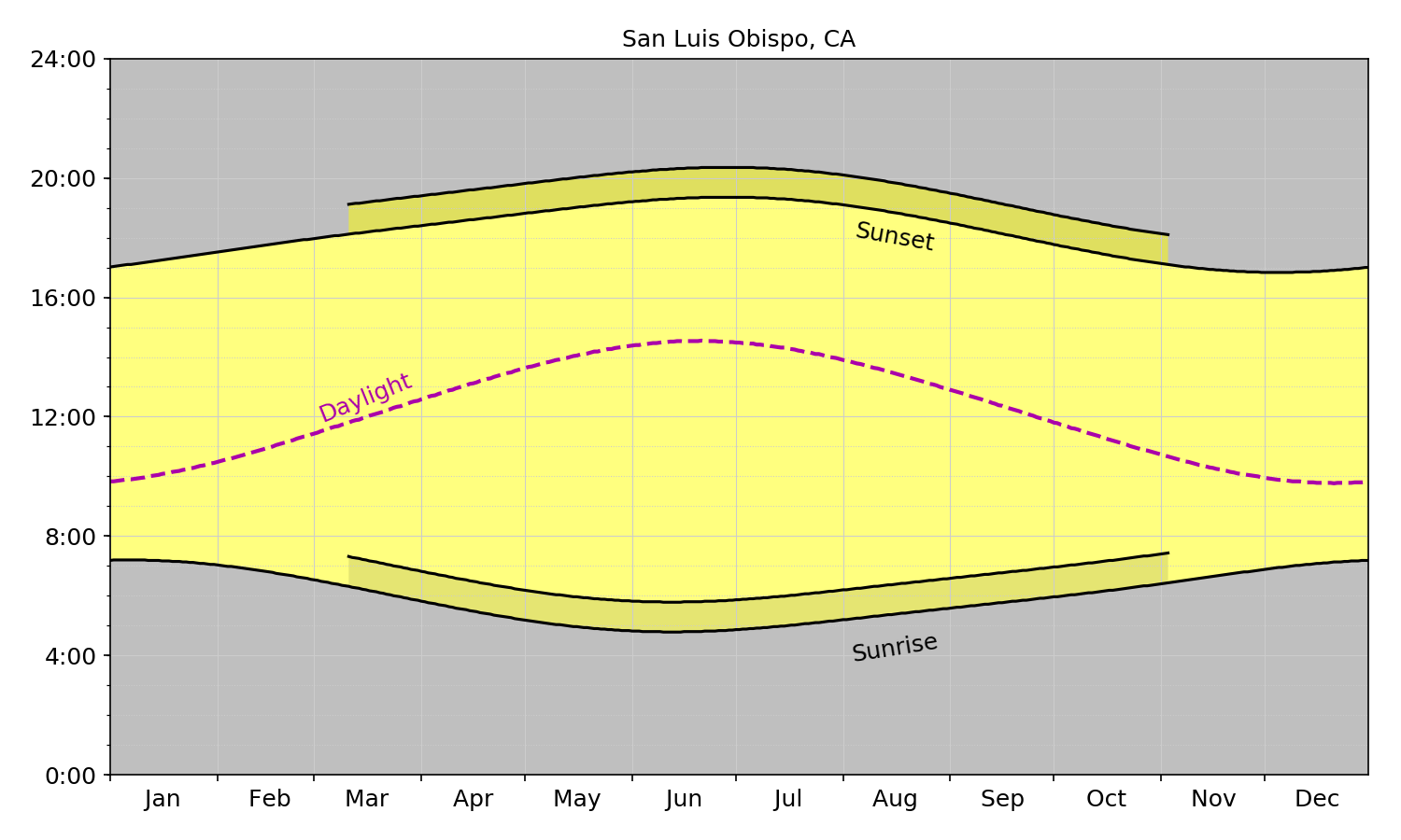
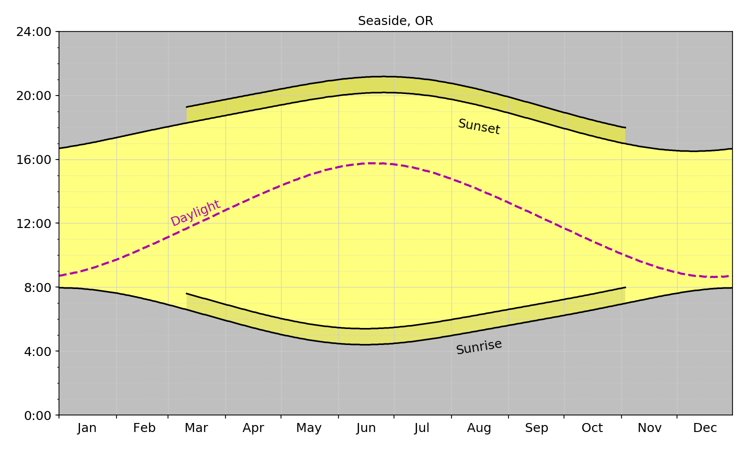
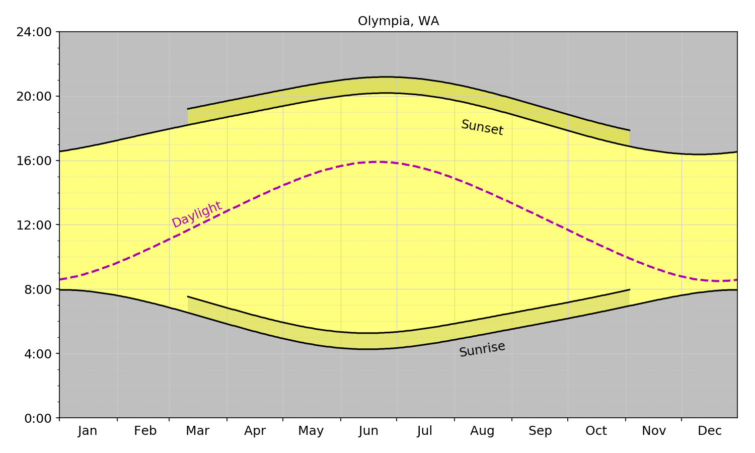
In the post he generated a chart showing both the total number of daylight hours and the sunrise / sunset times in Chicago. However, initially he didn’t post the code on how he generated it. The next day, in a follow up post, he did and that really got my thinking.

I wonder what the chart would look like for cities up and down the west coast (say from San Diego, CA to Seattle WA)?

Drang’s post had all of the code necessary to generate the graph, but for the data munging, he indicated:

If I were going to do this sort of thing on a regular basis, I’d write a script to handle this editing, but for a one-off I just did it “by hand.”

Doing it by hand wasn’t going to work for me if I was going to do several cities and so I needed to write a parser for the source of the data (The US Naval Observatory).

The entire script is on my GitHub sunrisesunset repo. I won’t go into the nitty gritty details, but I will call out a couple of things that I discovered during the development process.

Writing a parser is hard. Like really hard. Each time I thought I had it, I didn’t. I was finally able to get the parser to work o cities with 01, 29,30, or 31 in their longitude / latitude combinations.

I generated the same graph as Dr. Drang for the following cities:

• Phoenix, AZ
• Eugene, OR
• Portland
• Salem, OR
• Seaside, OR
• Eureka, CA
• Indio, CA
• Long Beach, CA
• Monterey, CA
• San Diego, CA
• San Francisco, CA
• San Luis Obispo, CA
• Ventura, CA
• Ferndale, WA
• Olympia, WA
• Seattle, WA

Why did I pick a city in Arizona? They don’t do Daylight Savings and I wanted to have a comparison of what it’s like for them!

The charts in latitude order (from south to north) are below:

San Diego

Phoenix

Indio

Long Beach

Ventura

San Luis Obispo

Monterey

San Francisco

Eureka

Eugene

Salem

Portland

Seaside

Olympia

Seattle

Ferndale

While these images do show the different impact of Daylight Savings, I think the images are more compelling when shown as a GIF:

We see just how different the impacts of DST are on each city depending on their latitude.

One of Dr. Drang’s main points in support of DST is:

If, by the way, you think the solution is to stay on DST throughout the year, I can only tell you that we tried that back in the 70s and it didn’t turn out well. Sunrise here in Chicago was after 8:00 am, which put school children out on the street at bus stops before dawn in the dead of winter. It was the same on the East Coast. Nobody liked that.

I think that comment says more about our school system and less about the need for DST.

For this whole argument I’m way more on the side of CGP Grey who does a great job of explaining what Day Lights Time is.

I think we may want to start looking at a Universal Planetary time (say UTC) and base all activities on that regardless of where you are in the world. The only reason 5am seems early (to some people) is because we’ve collectively decided that 5am (depending on the time of the year) is either WAY before sunrise or just a bit before sunrise, but really it’s just a number.

If we used UTC in California (where I’m at) 5am would we 12pm. Normally 12pm would be lunch time, but that’s only a convention that we have constructed. It could just as easily be the crack of dawn as it could be lunch time.

Do I think a conversion like this will ever happen? No. I just really hope that at some point in the distant future when aliens finally come and visit us, we aren’t late (or them early) because we have such a wacky time system here.

Posted by ryan on Mon 26 March 2018

Michael Kennedy over at Talk Python had a sale on his courses over the holidays so I took the plunge and bought them all. I have been listening to the podcast for several months now so I knew that I wouldn’t mind listening to him talk during a course (which is important!).

The first course I watched was ‘Python Jumpstart by Building 10 Apps’. The apps were:

• App 1: Hello (you Pythonic) world
• App 2: Guess that number game
• App 3: Birthday countdown app
• App 4: Journal app and file I/O
• App 5: Real-time weather client
• App 6: LOLCat Factory
• App 7: Wizard Battle App
• App 8: File Searcher App
• App 9: Real Estate Analysis App
• App 10: Movie Search App

For each app you learn a specific set of skills related to either Python or writing ‘Pyhonic’ code. I think the best part was that since it was all self paced I was able to spend time where I wanted to exploring ideas and concepts that wouldn’t have been available in traditional classrooms.

Also, since I’m fully adulted it can be hard to find time to watch and interact with courses like this so being able to watch them when I wanted to was a bonus.

Hello (you Pythonic) world is what you would expect from any introductory course. You write the basic ‘Hello World’ script, but with a twist. For this app you interact with it so that it asks your name and then it will output ‘Hello username my name is HAL!’ … although because I am who I am HAL wasn’t the name in the course, it was jut the name I chose for the app.

My favorite app to build and use was the Wizard App (app 7). It is a text adventure influenced by dungeons and dragons and teaches about classes and inheritance an polymorphism. It ws pretty cool.

The version that you are taught to make only has 4 creatures and ends pretty quickly. I enhanced the game to have it randomly create up to 250 creatures (some of them poisonous) and you level up during the game so that you can feel like a real character in an RPG.

The journal application was interesting because I finally started to get my head wrapped around file I/o. I’m not sure why I’ve had such a difficult time internalizing the concept, but the course seemed to help me better understand what was going on in terms of file streaming and reading data to do a thing.

My overall experience with the course was super positive. I’m really glad that I watched it and have already started to try to use the things that I’ve learned to improve code I’ve previously written.

With all of the good, there is some not so good.

The course uses it’s own player, which is fine, but it’s missing some key features:

1. Time reaming
2. Speed controls (i.e. it only plays at one speed, 1x)

In addition, sometimes the player would need to be reloaded which could be frustrating.

Overall though it was a great course and I’m glad I was able to do it.

Next course: Mastering PyCharm!

Posted by ryan on Tue 20 March 2018

In a previous post I wrote about my Raspberry Pi experiment to have the SenseHat display a scrolling message 10 minutes before game time.

One of the things I have wanted to do since then is have Vin Scully’s voice come from a speaker and say those five magical words, It's time for Dodger Baseball!

I found a clip of Vin on Youtube saying that (and a little more). I wasn’t sure how to get the audio from that YouTube clip though.

After a bit of googling¹ I found a command line tool called youtube-dl. The tool allowed me to download the video as an mp4 with one simple command:

youtube-dl https://www.youtube.com/watch?v=4KwFuGtGU6c

Once the mp4 was downloaded I needed to extract the audio from the mp4 file. Fortunately, ffmpeg is a tool for just this type of exercise!

I modified this answer from StackOverflow to meet my needs

ffmpeg -i dodger_baseball.mp4 -ss 00:00:10 -t 00:00:9.0 -q:a 0 -vn -acodec copy dodger_baseball.aac

This got me an aac file, but I was going to need an mp3 to use in my Python script.

Next, I used a modified version of this suggestion to create write my own command

ffmpeg -i dodger_baseball.aac -c:a libmp3lame -ac 2 -b:a 190k dodger_baseball.mp3

I could have probably combined these two steps, but … meh.

OK. Now I have the famous Vin Scully saying the best five words on the planet.

All that’s left to do is update the python script to play it. Using guidance from here I updated my itfdb.py file from this:

if month_diff == 0 and day_diff == 0 and hour_diff == 0 and 0 >= minute_diff >= -10:
   message = '#ITFDB!!! The Dodgers will be playing {} at {}'.format(game.game_opponent, game.game_time)
   sense.show_message(message, scroll_speed=0.05)

To this:

if month_diff == 0 and day_diff == 0 and hour_diff == 0 and 0 >= minute_diff >= -10:
   message = '#ITFDB!!! The Dodgers will be playing {} at {}'.format(game.game_opponent, game.game_time)
   sense.show_message(message, scroll_speed=0.05)
   os.system("omxplayer -b /home/pi/Documents/python_projects/itfdb/dodger_baseball.mp3")

However, what that does is play Vin’s silky smooth voice every minute for 10 minutes before game time. Music to my ears but my daughter was not a fan, and even my wife who LOVES Vin asked me to change it.

One final tweak, and now it only plays at 5 minutes before game time and 1 minute before game time:

if month_diff == 0 and day_diff == 0 and hour_diff == 0 and 0 >= minute_diff >= -10:
   message = '#ITFDB!!! The Dodgers will be playing {} at {}'.format(game.game_opponent, game.game_time)
   sense.show_message(message, scroll_speed=0.05)

if month_diff == 0 and day_diff == 0 and hour_diff == 0 and (minute_diff == -1 or minute_diff == -5):
   os.system("omxplayer -b /home/pi/Documents/python_projects/itfdb/dodger_baseball.mp3")

Now, for the rest of the season, even though Vin isn’t calling the games, I’ll get to hear his voice letting me know, “It’s Time for Dodger Baseball!!!”

1. Actually, it was an embarrassing amount ↩︎

Posted by ryan on Thu 15 March 2018

In my last post I indicated that I may need to

reinstalling everything on the Pi and starting from scratch

While speaking about my issues with pip3 and python3. Turns out that the fix was easier than I though. I checked to see what where pip3 and python3 where being executed from by running the which command.

The which pip3 returned /usr/local/bin/pip3 while which python3 returned /usr/local/bin/python3. This is exactly what was causing my problem.

To verify what version of python was running, I checked python3 --version and it returned 3.6.0.

To fix it I just ran these commands to unlink the new, broken versions:

sudo unlink /usr/local/bin/pip3

And

sudo unlink /usr/local/bin/python3

I found this answer on StackOverflow and tweaked it slightly for my needs.

Now, when I run python --version I get 3.4.2 instead of 3.6.0

Unfortunately I didn’t think to run the --version flag on pip before and after the change, and I’m hesitant to do it now as it’s back to working.

Posted by ryan on Tue 13 February 2018

In my last post I indicated that I may need to

reinstalling everything on the Pi and starting from scratch

While speaking about my issues with pip3 and python3. Turns out that the fix was easier than I though. I checked to see what where pip3 and python3 where being executed from by running the which command.

The which pip3 returned /usr/local/bin/pip3 while which python3 returned /usr/local/bin/python3. This is exactly what was causing my problem.

To verify what version of python was running, I checked python3 --version and it returned 3.6.0.

To fix it I just ran these commands to unlink the new, broken versions:

sudo unlink /usr/local/bin/pip3

And

sudo unlink /usr/local/bin/python3

I found this answer on StackOverflow and tweaked it slightly for my needs.

Now, when I run python --version I get 3.4.2 instead of 3.6.0

Unfortunately I didn’t think to run the --version flag on pip before and after the change, and I’m hesitant to do it now as it’s back to working.

Posted by ryan on Tue 13 February 2018

My wife and I love baseball season. Specifically we love the Dodgers and we can’t wait for Spring Training to begin. In fact, today pitchers and catchers report!

I’ve wanted to do something with the Raspberry Pi Sense Hat that I got (since I got it) but I’ve struggled to find anything useful. And then I remembered baseball season and I thought, ‘Hey, what if I wrote something to have the Sense Hat say “#ITFDB” starting 10 minutes before a Dodgers game started?’

And so I did!

The script itself is relatively straight forward. It reads a csv file and checks to see if the current time in California is within 10 minutes of start time of the game. If it is, then it will send a show_message command to the Sense Hat.

I also wrote a cron job to run the script every minute so that I get a beautiful scrolling bit of text every minute before the Dodgers start!

The code can be found on my GitHub page in the itfdb repository. There are 3 files:

1. Program.py which does the actual running of the script
2. data_types.py which defines a class used in Program.py
3. schedule.csv which is the schedule of the games for 2018 as a csv file.

I ran into a couple of issues along the way. First, my development environment on my Mac Book Pro was Python 3.6.4 while the Production Environment on the Raspberry Pi was 3.4. This made it so that the code about time ran locally but not on the server 🤦‍♂️.

It took some playing with the code, but I was finally able to go from this (which worked on 3.6 but not on 3.4):

now = utc_now.astimezone(pytz.timezone("America/Los_Angeles"))
game_date_time = game_date_time.astimezone(pytz.timezone("America/Los_Angeles"))

To this which worked on both:

local_tz = pytz.timezone('America/Los_Angeles')
now = utc_now.astimezone(local_tz)
game_date_time = local_tz.localize(game_date_time)

For both, the game_date_time variable setting was done in a for loop.

Another issue I ran into was being able to display the message for the sense hat on my Mac Book Pro. I wasn’t ever able to because of a package that is missing (RTIMU ) and is apparently only available on Raspbian (the OS on the Pi).

Finally, in my attempts to get the code I wrote locally to work on the Pi I decided to install Python 3.6.0 on the Pi (while 3.4 was installed) and seemed to do nothing but break pip. It looks like I’ll be learning how to uninstall Python 3.4 OR reinstalling everything on the Pi and starting from scratch. Oh well … at least it’s just a Pi and not a real server.

Although, I’m pretty sure I hosed my Linode server a while back and basically did the same thing so maybe it’s just what I do with servers when I’m learning.

One final thing. While sitting in the living room watching DC Legends of Tomorrow the Sense Hat started to display the message. Turns out, I was accounting for the minute, hour, and day but NOT the month. The Dodgers play the Cubs on September 12 at 9:35 (according to the schedule.csv file anyway) and so the conditions to display were met.

I added another condition to make sure it was the right month and now we’re good to go!

Super pumped for this season with the Dodgers!

Posted by ryan on Tue 13 February 2018

My wife and I love baseball season. Specifically we love the Dodgers and we can’t wait for Spring Training to begin. In fact, today pitchers and catchers report!

I’ve wanted to do something with the Raspberry Pi Sense Hat that I got (since I got it) but I’ve struggled to find anything useful. And then I remembered baseball season and I thought, ‘Hey, what if I wrote something to have the Sense Hat say “#ITFDB” starting 10 minutes before a Dodgers game started?’

And so I did!

The script itself is relatively straight forward. It reads a csv file and checks to see if the current time in California is within 10 minutes of start time of the game. If it is, then it will send a show_message command to the Sense Hat.

I also wrote a cron job to run the script every minute so that I get a beautiful scrolling bit of text every minute before the Dodgers start!

The code can be found on my GitHub page in the itfdb repository. There are 3 files:

1. Program.py which does the actual running of the script
2. data_types.py which defines a class used in Program.py
3. schedule.csv which is the schedule of the games for 2018 as a csv file.

I ran into a couple of issues along the way. First, my development environment on my Mac Book Pro was Python 3.6.4 while the Production Environment on the Raspberry Pi was 3.4. This made it so that the code about time ran locally but not on the server 🤦‍♂️.

It took some playing with the code, but I was finally able to go from this (which worked on 3.6 but not on 3.4):

now = utc_now.astimezone(pytz.timezone("America/Los_Angeles"))
game_date_time = game_date_time.astimezone(pytz.timezone("America/Los_Angeles"))

To this which worked on both:

local_tz = pytz.timezone('America/Los_Angeles')
now = utc_now.astimezone(local_tz)
game_date_time = local_tz.localize(game_date_time)

For both, the game_date_time variable setting was done in a for loop.

Another issue I ran into was being able to display the message for the sense hat on my Mac Book Pro. I wasn’t ever able to because of a package that is missing (RTIMU ) and is apparently only available on Raspbian (the OS on the Pi).

Finally, in my attempts to get the code I wrote locally to work on the Pi I decided to install Python 3.6.0 on the Pi (while 3.4 was installed) and seemed to do nothing but break pip. It looks like I’ll be learning how to uninstall Python 3.4 OR reinstalling everything on the Pi and starting from scratch. Oh well … at least it’s just a Pi and not a real server.

Although, I’m pretty sure I hosed my Linode server a while back and basically did the same thing so maybe it’s just what I do with servers when I’m learning.

One final thing. While sitting in the living room watching DC Legends of Tomorrow the Sense Hat started to display the message. Turns out, I was accounting for the minute, hour, and day but NOT the month. The Dodgers play the Cubs on September 12 at 9:35 (according to the schedule.csv file anyway) and so the conditions to display were met.

I added another condition to make sure it was the right month and now we’re good to go!

Super pumped for this season with the Dodgers!

Posted by ryan on Tue 13 February 2018

In my last post I wrote out the steps that I was going to use to turn a ton of .h264 files into one mp4 file with the use of MP4Box.

Before outlining my steps I said, “The method below works but I’m sure that there is a better way to do it.”

Shortly after posting that I decided to find that better way. Turns out, ~~it wasn’t really that much more work~~ it was much harder than originally thought.

The command below is a single line and it will create a text file (com.txt) and then execute it as a bash script:

~~(echo '#!/bin/sh'; for i in *.h264; do if [ "$i" -eq 1 ]; then echo -n " -add $i"; else echo -n " -cat $i"; fi; done; echo -n " hummingbird.mp4") > /Desktop/com.txt | chmod +x /Desktop/com.txt | ~/Desktop/com.txt~~

(echo '#!/bin/sh'; echo -n "MP4Box"; array=($(ls *.h264)); for index in ${!array[@]}; do if [ "$index" -eq 1 ]; then echo -n " -add ${array[index]}"; else echo -n " -cat ${array[index]}"; fi; done; echo -n " hummingbird.mp4") > com.txt | chmod +x com.txt

Next you execute the script with

./com.txt

OK, but what is it doing? The parentheses surround a set of echo commands that output to com.txt. I’m using a for loop with an if statement. The reason I can’t do a straight for loop is because the first h264 file used in MP4Box needs to have the -add flag while all of the others need the -cat flag.

Once the file is output to the com.txt file (on the Desktop) I pipe it to the chmod +x command to change it’s mode to make it executable.

Finally, I pipe that to a command to run the file ~/Desktop/com.txt

I was pretty stoked when I figured it out and was able to get it to run.

The next step will be to use it for the hundreds of h264 files that will be output from my hummingbird camera that I just installed today.

I’ll have a post on that in the next couple of days.

Posted by ryan on Sat 10 February 2018

The general form of the concatenate command for MP4Box is:

MP4Box -add <filename>.ext -cat <filename>.ext output.ext¹

When you have more than a couple of output files, you’re going to want to automate that -cat part as much as possible because let’s face it, writing out that statement even more than a couple of times will get really old really fast.

The method below works but I’m sure that there is a better way to do it.

1. echo out the command you want to run. In this case:

(echo -n "MP4Box "; for i in *.h264; do echo -n " -cat $i"; done; echo -n " hummingbird.mp4") >> com.txt

1. Edit the file com.txt created in (1) so that you can change the first -cat to -add

vim com.txt

1. While still in vim editing the com.txt file add the #!/bin/sh to the first line. When finished, exit vim²
2. Change the mode of the file so it can run

chmod +x com.txt

1. Run the file:

./com.txt

Why am I doing all of this? I have a Raspberry Pi with a Camera attachment and a motion sensor. I’d like to watch the hummingbirds that come to my hummingbird feeder with it for a day or two and get some sweet video. We’ll see how it goes.

1. The -add will add the \<filename> to the output file while the -cat will add any other files to the output file (all while not overwriting the output file so that the files all get streamed together). ↩︎
2. I’m sure there’s an xkcd comic about this, but I just can’t find it! ↩︎

Posted by ryan on Thu 08 February 2018

I’d discovered a python package called osmnx which will take GIS data and allow you to draw maps using python. Pretty cool, but I wasn’t sure what I was going to do with it.

After a bit of playing around with it I finally decided that I could make some pretty cool Fractures.

I’ve got lots of Fracture images in my house and I even turned my diplomas into Fractures to hang up on the wall at my office, but I hadn’t tried to make anything like this before.

I needed to figure out what locations I was going to do. I decided that I wanted to do 9 of them so that I could create a 3 x 3 grid of these maps.

I selected 9 cities that were important to me and my family for various reasons.

Next writing the code. The script is 54 lines of code and doesn’t really adhere to PEP8 but that just gives me a chance to do some reformatting / refactoring later on.

In order to get the desired output I needed several libraries:

osmnx (as I’d mentioned before)
matplotlib.pyplot
numpy
PIL

If you’ve never used PIL before it’s the ‘Python Image Library’ and according to it’s home page it

adds image processing capabilities to your Python interpreter. This library supports many file formats, and provides powerful image processing and graphics capabilities.

OK, let’s import some libraries!

import osmnx as ox, geopandas as gpd, os
import matplotlib.pyplot as plt
import numpy as np
from PIL import Image
from PIL import ImageFont
from PIL import ImageDraw

Next, we establish the configurations:

ox.config(log_file=True, log_console=False, use_cache=True)

The ox.config allows you to specify several options. In this case, I’m:

1. Specifying that the logs be saved to a file in the log directory
2. Suppress the output of the log file to the console (this is helpful to have set to True when you’re first running the script to see what, if any, errors you have.
3. The use_chache=True will use a local cache to save/retrieve http responses instead of calling API repetitively for the same request URL

This option will help performance if you have the run the script more than once.

OSMX has many different options to generate maps. I played around with the options and found that the walking network within 750 meters of my address gave me the most interesting lines.

AddressDistance = 750
AddressDistanceType = 'network'
AddressNetworkType = 'walk'

Now comes some of the most important decisions (and code!). Since I’ll be making this into a printed image I want to make sure that the image and resulting file will be of a high enough quality to render good results. I also want to start with a white background (although a black background might have been kind of cool). I also want to have a high DPI. Taking these needs into consideration I set my plot variables:

PlotBackgroundColor = '#ffffff'
PlotNodeSize = 0
PlotFigureHeight = 40
PlotFigureWidth = 40
PlotFileType = 'png'
PlotDPI = 300
PlotEdgeLineWidth = 10.0

I played with the PlotEdgeLineWidth a bit until I got a result that I liked. It controls how thick the route lines are and is influenced by the PlotDPI. For the look I was going for 10.0 worked out well for me. I’m not sure if that means a 30:1 ratio for PlotDPI to PlotEdgeLineWidth would be universal but if you like what you see then it’s a good place to start.

One final piece was deciding on the landmarks that I was going to use. I picked nine places that my family and I had been to together and used addresses that were either of the places that we stayed at (usually hotels) OR major landmarks in the areas that we stayed. Nothing special here, just a text file with one location per line set up as

Address, City, State

For example:

1234 Main Street, Anytown, CA

So we just read that file into memory:

landmarks = open('/Users/Ryan/Dropbox/Ryan/Python/landmarks.txt', 'r')

Next we set up some scaffolding so we can loop through the data effectively

landmarks = landmarks.readlines()
landmarks = [item.rstrip() for item in landmarks]

fill = (0,0,0,0)

city = []

The loop below is doing a couple of things:

1. Splits the landmarks array into base elements by breaking it apart at the commas (I can do this because of the way that the addresses were entered. Changes may be needed to account for my complex addresses (i.e. those with multiple address lines (suite numbers, etc) or if local addresses aren’t constructed in the same way that US addresses are)
2. Appends the second and third elements of the parts array and replaces the space between them with an underscore to convert Anytown, CA to Anytown_CA

<!-- -->

for element in landmarks:
    parts = element.split(',')
    city.append(parts[1].replace(' ', '', 1)+'_'+parts[2].replace(' ', ''))

This next line isn’t strictly necessary as it could just live in the loop, but it was helpful for me when writing to see what was going on. We want to know how many items are in the landmarks

rows = len(landmarks)

Now to loop through it. A couple of things of note:

The package includes several graph_from_... functions. They take as input some type, like address, i.e. graph_from_address (which is what I’m using) and have several keyword arguments.

In the code below I’m using the ith landmarks item and setting the distance, distance_type, network_type and specifying an option to make the map simple by setting simplify=‘true’

To add some visual interest to the map I’m using this line

ec = ['#cc0000' if data['length'] >=100 else '#3366cc' for u, v, key, data in G.edges(keys=True, data=True)]

If the length of the part of the map is longer than 100m then the color is displayed as #cc0000 (red) otherwise it will be #3366cc (blue)

The plot_graph is what does the heavy lifting to generate the image. It takes as input the output from the graph_from_address and ec to identify what and how the map will look.

Next we use the PIL library to add text to the image. It takes into memory the image file and saves out to a directory called /images/. My favorite part of this library is that I can choose what font I want to use (whether it’s part of the system fonts or a custom user font) and the size of the font. For my project I used San Francisco at 512.

Finally, there is an exception for the code that adds text. The reason for this is that when I was playing with adding text to the image I found that for 8 of 9 maps having the text in the upper left hand corner worker really well. It was just that last one (San Luis Obispo, CA) that didn’t.

So, instead of trying to find a different landmark, I decided to take a bit of artistic license and put the San Luis Obispo text in the upper right hard corner.

Once the script is all set simply typing python MapProject.py in my terminal window from the directory where the file is saved generated the files.

All I had to do what wait and the images were saved to my /images/ directory.

Next, upload to Fracture and order the glass images!

I received the images and was super excited. However, upon opening the box and looking at them I noticed something wasn’t quite right

[caption id="attachment_188" align="alignnone" width="2376"]![Napa with the text slightly off the image]images/uploads/2018/01/Image-12-16-17-6-55-AM.jpeg){.alignnone .size-full .wp-image-188 width="2376" height="2327"} Napa with the text slightly off the image[/caption]

As you can see, the name place is cut off on the left. Bummer.

No reason to fret though! Fracture has a 100% satisfaction guarantee. So I emailed support and explained the situation.

Within a couple of days I had my bright and shiny fractures to hang on my wall

[caption id="attachment_187" align="alignnone" width="2138"]![Napa with the text properly displaying]images/uploads/2018/01/IMG_9079.jpg){.alignnone .size-full .wp-image-187 width="2138" height="2138"} Napa with the text properly displaying[/caption]

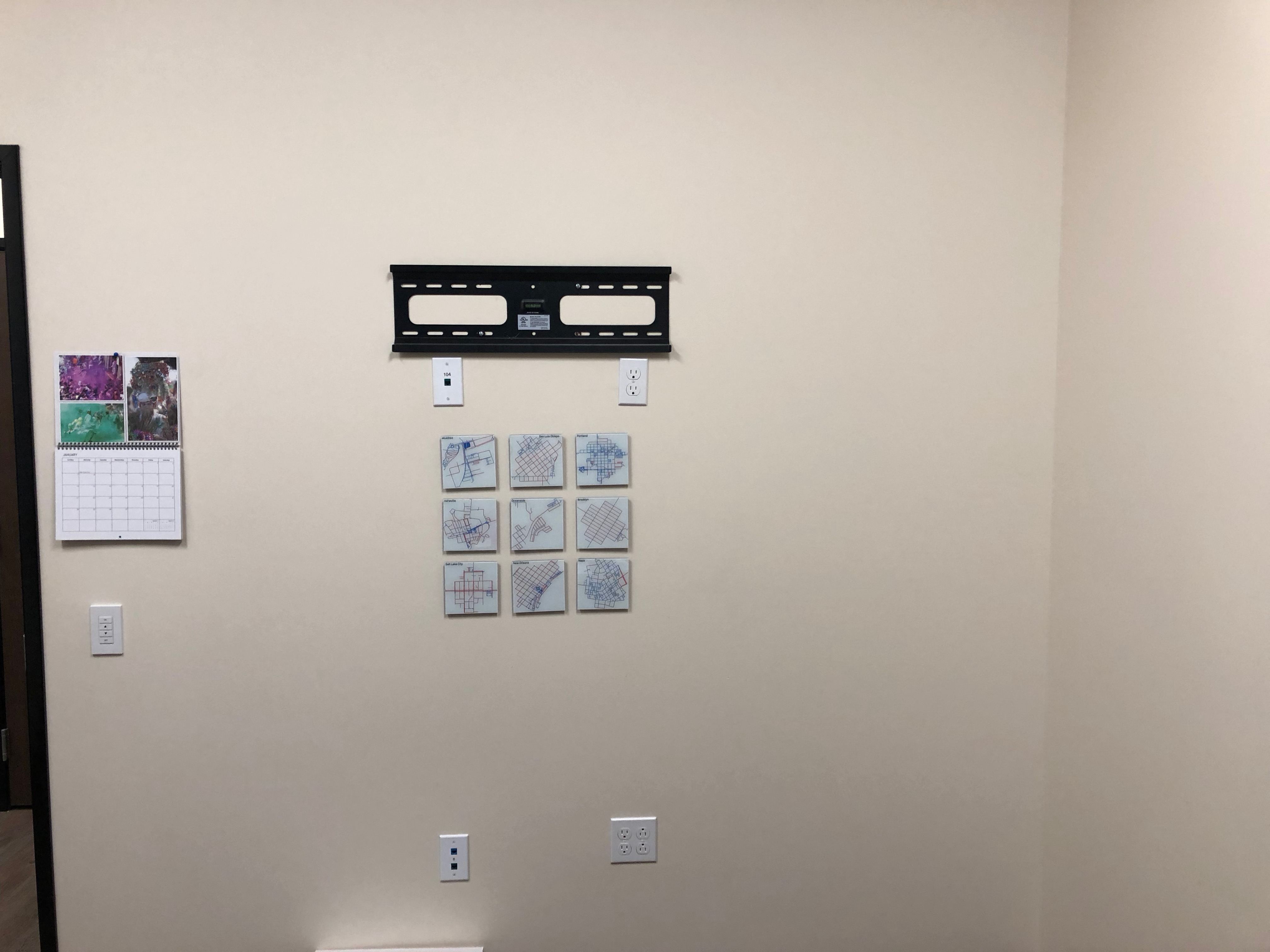
So that my office wall is no longer blank and boring:

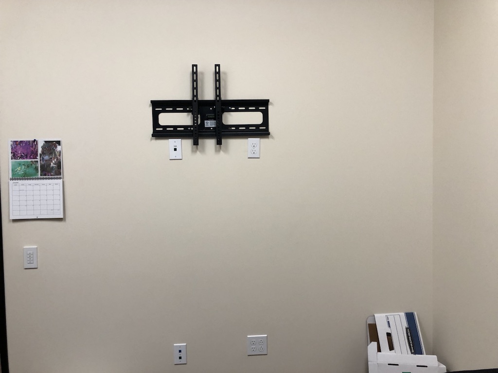
but interesting and fun to look at

Posted by ryan on Fri 12 January 2018