One of the great things about computers is their ability to take tabular data and turn them into pictures that are easier to interpret. I'm always amazed when given the opportunity to show data as a picture, more people don't jump at the chance.

For example, this piece on ESPN regarding the difference in officiating crews and their calls has some great data in it regarding how different officiating crews call games.

One thing I find a bit disconcerting is:

1. ~~One of the rows is missing data so that row looks 'odd' in the context of the story and makes it look like the writer missed a big thing ... they didn't~~ (it's since been fixed)
2. This tabular format is just begging to be displayed as a picture.

Perhaps the issue here is that the author didn't know how to best visualize the data to make his story, but I'm going to help him out.

If we start from the underlying premise that not all officiating crews call games in the same way, we want to see in what ways they differ.

The data below is a reproduction of the table from the article:

REFEREE DEF. OFFSIDE ENCROACH FALSE START NEUTRAL ZONE TOTAL

Triplette, Jeff 39 2 34 6 81 Anderson, Walt 12 2 39 10 63 Blakeman, Clete 13 2 41 7 63 Hussey, John 10 3 42 3 58 Cheffers, Cartlon 22 0 31 3 56 Corrente, Tony 14 1 31 8 54 Steratore, Gene 19 1 29 5 54 Torbert, Ronald 9 4 31 7 51 Allen, Brad 15 1 28 6 50 McAulay, Terry 10 4 23 12 49 Vinovich, Bill 8 7 29 5 49 Morelli, Peter 12 3 24 9 48 Boger, Jerome 11 3 27 6 47 Wrolstad, Craig 9 1 31 5 46 Hochuli, Ed 5 2 33 4 44 Coleman, Walt 9 2 25 4 40 Parry, John 7 5 20 6 38

The author points out:

Jeff Triplette's crew has called a combined 81 such penalties -- 18 more than the next-highest crew and more than twice the amount of two others

The author goes on to talk about his interview with Mike Pereira (who happens to be ~~pimping~~ promoting his new book).

While the table above is helpful it's not an image that you can look at and ask, "Man, what the heck is going on?" There is a visceral aspect to it that says, something is wrong here ... but I can't really be sure about what it is.

Let's sum up the defensive penalties (Defensive Offsides, Encroachment, and Neutral Zone Infractions) and see what the table looks like:

REFEREE DEF Total OFF Total TOTAL

Triplette, Jeff 47 34 81 Anderson, Walt 24 39 63 Blakeman, Clete 22 41 63 Hussey, John 16 42 58 Cheffers, Cartlon 25 31 56 Corrente, Tony 23 31 54 Steratore, Gene 25 29 54 Torbert, Ronald 20 31 51 Allen, Brad 22 28 50 McAulay, Terry 26 23 49 Vinovich, Bill 20 29 49 Morelli, Peter 24 24 48 Boger, Jerome 20 27 47 Wrolstad, Craig 15 31 46 Hochuli, Ed 11 33 44 Coleman, Walt 15 25 40 Parry, John 18 20 38

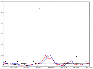
Now we can see what might actually be going on, but it's still a bit hard for those visual people. If we take this data and then generate a scatter plot we might have a picture to show us the issue. Something like this:

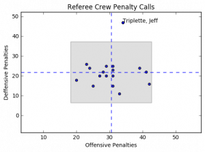
The horizontal dashed blue lines represent the average defensive calls per crew while the vertical dashed blue line represents the average offensive calls per crew. The gray box represents the area containing plus/minus 2 standard deviations from the mean for both offensive and defensive penalty calls.

Notice anything? Yeah, me too. Jeff Triplette's crew is so far out of range for defensive penalties it's like they're watching a different game, or reading from a different play book.

What I'd really like to be able to do is this same analysis but on a game by game basis. I don't think this would really change the way that Jeff Triplette and his crew call games, but it may point out some other inconsistencies that are worth exploring.

Code for this project can be found on my GitHub Repo

Posted by ryan on Sun 25 December 2016

I have a 10 year old daughter in the fifth grade. She has participated in the Science Fair almost every year, but this year was different. This year was required participation.

dun … dun … dun …

She and her friend had a really interesting idea on what to do. They wanted to ask the question, “Is Soap and Water the Best Cleaning Method?”

The two Scientists decided that they would test how well the following cleaning agents cleaned a white t-shirt (my white t-shirt actually) after it got dirty:

• Plain Water
• Soap and Water
• Milk
• Almond Milk

While working with them we experimented on how to make the process as scientific as possible. Our first attempt was to just take a picture of the Clean shirt, cut the shirt up and get it dirty. Then we’d try each cleaning agent to see how it went.

It did not go well. It was immediately apparent that there would be no way to test the various cleaning methods efficacy.

No problem. In our second trial we decided to approach it more scientifically.

We would draw 12 equally sized squares on the shirt and take a picture:

We needed 12 squares because we had 4 cleaning methods and 3 trials that needed to be performed

4 Cleaning Methods X 3 Trials = 12 Samples

Next, the Scientists would get the shirt dirty. We then cut out the squares so that we could test cleaning the samples.

Here’s an outline of what the Scientists did to test their hypothesis:

1. Take a picture of each piece BEFORE they get dirty
2. Get each sample dirty
3. Take a picture of each dirty sample
4. Clean each sample
5. Take a picture of each cleaned sample
6. Repeat for each trial

For the ‘Clean Each Sample’ step they placed 1/3 of a cup of the cleaning solution into a small Tupperware tub that could be sealed and vigorously shook for 5 minutes. They had some tired arms at the end.

Once we had performed the experiment we our raw data:

Trial 1

Method Start Dirty Cleaned

Water Soap And Water Milk Almond Milk

Trial 2

Method Start Dirty Cleaned

Water Soap And Water Milk Almond Milk

Trial 3

Method Start Dirty Cleaned

Water Soap And Water Milk Almond Milk

This is great and all, but now what? We can’t really use subjective measures to determine cleanliness and call it science!

My daughter and her friend aren’t coders, but I did explain to them that we needed a more scientific way to determine cleanliness. I suggested that we use python to examine the image and determine the brightness of the image.

We could then use some math to compare the brightness. ¹

Now, onto the code!

OK, let’s import some libraries:

from PIL import Image, ImageStat
import math
import glob
import pandas as pd
import matplotlib.pyplot as plt

There are 2 functions to determine brightness that I found here. They were super useful for this project. As an aside, I love StackOverflow!

#Convert image to greyscale, return average pixel brightness.
def brightness01( im_file ):
   im = Image.open(im_file).convert('L')
   stat = ImageStat.Stat(im)
   return stat.mean[0]

#Convert image to greyscale, return RMS pixel brightness.
def brightness02( im_file ):
   im = Image.open(im_file).convert('L')
   stat = ImageStat.Stat(im)
   return stat.rms[0]

The next block of code takes the images and processes them to get the return the brightness levels (both of them) and return them to a DataFrame to be used to write to a csv file.

I named the files in such a way so that I could automate this. It was a bit tedious (and I did have the scientists help) but they were struggling to understand why we were doing what we were doing. Turns out teaching CS concepts is harder than it looks.

f = []
img_brightness01 = []
img_brightness02 = []
trial = []
state = []
method = []
for filename in glob.glob('/Users/Ryan/Dropbox/Abby/Science project 2016/cropped images/**/*', recursive=True):
    f.append(filename.split('/')[-1])
    img_brightness01.append(round(brightness01(filename),0))
    img_brightness02.append(round(brightness02(filename),0))
for part in f:
    trial.append(part.split('_')[0])
    state.append(part.split('_')[1])
    method.append(part.split('_')[2].replace('.png', '').replace('.jpg',''))

dic = {'TrialNumber': trial, 'SampleState': state, 'CleaningMethod': method, 'BrightnessLevel01': img_brightness01, 'BrightnessLevel02': img_brightness02}

results = pd.DataFrame(dic)

I’m writing the output to a csv file here so that the scientist will have their data to make their graphs. This is where my help with them ended.

#write to a csv file
results.to_csv('/Users/Ryan/Dropbox/Abby/Science project 2016/results.csv')

Something I wanted to do though was to see what our options were in python for creating graphs. Part of the reason this wasn’t included with the science project is that we were on a time crunch and it was easier for the Scientists to use Google Docs to create their charts, and part of it was that I didn’t want to cheat them out of creating the charts on their own.

There is a formula below to determine a score which is given by a normalized percentage that was used by them, but the graphing portion below I did after the project was turned in.

Let’s get the setup out of the way:

#Create Bar Charts
trials = ['Trial1','Trial2','Trial3']

n_trials = len(trials)
index = np.arange(n_trials)
bar_width = 0.25
bar_buffer = 0.05
opacity = 0.4

graph_color = ['b', 'r', 'g', 'k']
methods = ['Water', 'SoapAndWater', 'Milk', 'AlmondMilk']

graph_data = []

Now, let’s loop through each cleaning method and generate a list of scores (where one score is for one trial)

for singlemethod in methods:
    score= []
    for trialnumber in trials:
        s = results.loc[results['CleaningMethod'] == singlemethod].loc[results['TrialNumber'] == trialnumber].loc[results['SampleState'] == 'Start'][['BrightnessLevel01']]
        s = list(s.values.flatten())[0]
        d = results.loc[results['CleaningMethod'] == singlemethod].loc[results['TrialNumber'] == trialnumber].loc[results['SampleState'] == 'Dirty'][['BrightnessLevel01']]
        d = list(d.values.flatten())[0]
        c = results.loc[results['CleaningMethod'] == singlemethod].loc[results['TrialNumber'] == trialnumber].loc[results['SampleState'] == 'Clean'][['BrightnessLevel01']]
        c = list(c.values.flatten())[0]
        scorepct =  float((c-d) / (s - d))
        score.append(scorepct)
    graph_data.append(score)

This last section was what stumped me for the longest time. I had such a mental block converting from iterating over items in a list to item counts of a list. After much Googling I was finally able to make the breakthrough I needed and found the idea of looping through a range and everything came together:

for i in range(0, len(graph_data)):
    plt.bar(index+ (bar_width)*i, graph_data[i], bar_width-.05, alpha=opacity,color=graph_color[i],label=methods[i])
    plt.xlabel('Trial Number')
    plt.axvline(x=i-.025, color='k', linestyle='--')
    plt.xticks(index+bar_width*2, trials)
    plt.yticks((-1,-.75, -.5, -.25, 0,0.25, 0.5, 0.75, 1))
    plt.ylabel('Brightness Percent Score')
    plt.title('Comparative Brightness Scores')
    plt.legend(loc=3)

The final output of this code gives:

From the graph you can see the results are … inconclusive. I’m not sure what the heck happened in Trial 3 but the Scientists were able to make the samples dirtier. Ignoring Trial 3 there is no clear winner in either Trial 1 or Trial 2.

I think it would have been interesting to have 30 - 45 trials and tested this with a some statistics, but that’s just me wanting to show something to be statistically valid.

I think the best part of all of this was the time I got to spend with my daughter and the thinking through the experiment. I think she and her friend learned a bit more about the scientific method (and hey, isn’t that what this type of thing is all about?).

I was also really excited when her friend said, “Science is pretty cool” and then had a big smile on her face.

They didn’t go onto district, or get a blue ribbon, but they won in that they learned how neat science can be.

1. [The score is the ratio of how clean the cleaning method was able to get the sample compared to where it started, i.e. the ratio of the difference of the cleaned sample and the dirty sample to the difference of the starting sample and the dirty sample. ↩︎

Posted by ryan on Sat 17 December 2016

In one of my previous posts I walked through how I generated a wordcloud based on my most recent 20 tweets. I though it would be neat to do this for my Dropbox file names as well. just to see if I could.

When I first tried to do it (as previously stated, the Twitter Word Cloud post was the first python script I wrote) I ran into some difficulties. I didn't really understand what I was doing (although I still don't really understand, I at least have a vague idea of what the heck I'm doing now).

The script isn't much different than the Twitter word cloud. The only real differences are:

1. the way in which the words variable is being populated
2. the mask that I'm using to display the cloud

In order to go get the information from the file system I use the glob library:

import glob

The next lines have not changed

import matplotlib.pyplot as plt
from wordcloud import WordCloud, STOPWORDS
from scipy.misc import imread

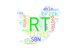
Instead of writing to a 'tweets' file I'm looping through the files, splitting them at the / character and getting the last item (i.e. the file name) and appending it to the list f:

f = []
for filename in glob.glob('/Users/Ryan/Dropbox/Ryan/**/*', recursive=True):
    f.append(filename.split('/')[-1])

The rest of the script generates the image and saves it to my Dropbox Account. Again, instead of using a Twitter logo, I'm using a Cloud image I found here

words = ' '
for line in f:
    words= words + line

stopwords = {'https'}

logomask = imread('mask-cloud.png')

wordcloud = WordCloud(
    font_path='/Users/Ryan/Library/Fonts/Inconsolata.otf',
    stopwords=STOPWORDS.union(stopwords),
    background_color='white',
    mask = logomask,
    max_words=1000,
    width=1800,
    height=1400
).generate(words)

plt.imshow(wordcloud.recolor(color_func=None, random_state=3))
plt.axis('off')
plt.savefig('/Users/Ryan/Dropbox/Ryan/Post Images/dropbox_wordcloud.png', dpi=300)
plt.show()

And we get this:

Posted by ryan on Fri 25 November 2016

I read about a cool gis package for Python and decided I wanted to play around with it. This post isn't about any of the things I've learned about the package, it's so I can remember how I installed it so I can do it again if I need to. The package is described by it's author in his post

To install osmnx I needed to do the following:

1. Install Home Brew if it's not already installed by running this command (as an administrator) in the terminal:

   /usr/bin/ruby -e "$(curl -fsSL https://raw.githubusercontent.com/Homebrew/install/master/install)"

2. Use Home Brew to install the spatialindex dependency. From the terminal (again as an administrator):

   brew install spatialindex

3. In python run pip to install rtree:

   pip install rtree

4. In python run pip to install osmnx

   pip install osmnx

I did this on my 2014 iMac but didn't document the process. This lead to a problem when I tried to run some code on my 2012 MacBook Pro.

Step 3 may not be required, but I'm not sure and I don't want to not have it written down and then wonder why I can't get osmnx to install in 3 years when I try again!

Remember, you're not going to remember what you did, so you need to write it down!

Posted by ryan on Thu 24 November 2016

As previously mentioned I'm a bit of a Twitter user. One of the things that I came across, actually the first python project I did, was writing code to create a word cloud based on the most recent 20 posts of my Twitter feed.

I used a post by Sebastian Raschka and a post on TechTrek.io as guides and was able to generate the word cloud pretty easily.

As usual, we import the need libraries:

import tweepy, json, random
from tweepy import OAuthHandler
import matplotlib.pyplot as plt
from wordcloud import WordCloud, STOPWORDS
from scipy.misc import imread

The code below allows access to my feed using secret keys from my twitter account. They have been removed from the post so that my twitter account doesn't stop being mine:

consumer_key = consumer_key
consumer_secret = consumer_secret
access_token = access_token
access_secret = access_secret

auth = OAuthHandler(consumer_key, consumer_secret)
auth.set_access_token(access_token, access_secret)

api = tweepy.API(auth)

Next I open a file called tweets and write to it the tweets (referred to in the for loop as status) and encode with utf-8. If you don't do the following error is thrown: TypeError: a bytes-like object is required, not 'str'. And who wants a TypeError to be thrown?

f = open('tweets', 'wb')

for status in api.user_timeline():
    f.write(api.get_status(status.id).text.encode("utf-8"))
f.close()

Now I'm ready to do something with the tweets that I collected. I read the file into a variable called words

words=' '
count =0
f = open('tweets', 'rb')
for line in f:
    words= words + line.decode("utf-8")
f.close

Next, we start on constructing the word cloud itself. We declare words that we want to ignore (in this case https is ignored, otherwise it would count the protocol of links that I've been tweeting).

stopwords = {'https', 'co', 'RT'}

Read in the twitter bird to act as a mask

logomask = imread('twitter_mask.png')

Finally, generate the wordcloud, plot it and save the image:

wordcloud = WordCloud(
    font_path='/Users/Ryan/Library/Fonts/Inconsolata.otf',
    stopwords=STOPWORDS.union(stopwords),
    background_color='white',
    mask = logomask,
    max_words=500,
    width=1800,
    height=1400
).generate(words)

plt.imshow(wordcloud.recolor(color_func=None, random_state=3))
plt.axis('off')
plt.savefig('./Twitter Word Cloud - '+time.strftime("%Y%m%d")+'.png', dpi=300)
plt.show()

The second to last line generates a dynamically named file based on the date so that I can do this again and save the image without needing to do too much thinking.

Full Code can be found on my GitHub Report

My Twitter Word Cloud as of today looks like this:

I think it will be fun to post this image every once in a while, so as I remember, I'll run the script again and update the Word Cloud!

Posted by ryan on Wed 23 November 2016

I'm an avid Twitter user, mostly as a replacement RSS feeder, but also because I can't stand Facebook and this allows me to learn about really important world events when I need to and to just stay isolated with my head in the sand when I don't. It's perfect for me.

One of the people I follow on Twitter is Dr. Drang who is an Engineer of some kind by training. He also appears to be a fan of baseball and posted an analysis of Jake Arrieata's pitching over the course of the 2016 MLB season (through September 22 at least).

When I first read it I hadn't done too much with Python, and while I found the results interesting, I wasn't sure what any of the code was doing (not really anyway).

Since I had just spent the last couple of days learning more about BeautifulSoup specifically and Python in general I thought I'd try to do two things:

1. Update the data used by Dr. Drang
2. Try to generalize it for any pitcher

Dr. Drang uses a flat csv file for his analysis and I wanted to use BeautifulSoup to scrape the data from ESPN directly.

OK, I know how to do that (sort of ¯\(ツ)/¯)

First things first, import your libraries:

import pandas as pd
from functools import partial
import requests
import re
from bs4 import BeautifulSoup
import matplotlib.pyplot as plt
from datetime import datetime, date
from time import strptime

The next two lines I ~~stole~~ borrowed directly from Dr. Drang's post. The first line is to force the plot output to be inline with the code entered in the terminal. The second he explains as such:

The odd ones are the rcParams call, which makes the inline graphs bigger than the tiny Jupyter default, and the functools import, which will help us create ERAs over small portions of the season.

I'm not using Jupyter I'm using Rodeo as my IDE but I kept them all the same:

%matplotlib inline
plt.rcParams['figure.figsize'] = (12,9)

In the next section I use BeautifulSoup to scrape the data I want from ESPN:

url = 'http://www.espn.com/mlb/player/gamelog/_/id/30145/jake-arrieta'
r = requests.get(url)
year = 2016

date_pitched = []
full_ip = []
part_ip = []
earned_runs = []

tables = BeautifulSoup(r.text, 'lxml').find_all('table', class_='tablehead mod-player-stats')
for table in tables:
    for row in table.find_all('tr'): # Remove header
        columns = row.find_all('td')
        try:
            if re.match('[a-zA-Z]{3}\s', columns[0].text) is not None:
                date_pitched.append(
                    date(
                    year
                    , strptime(columns[0].text.split(' ')[0], '%b').tm_mon
                    , int(columns[0].text.split(' ')[1])
                    )
                )
                full_ip.append(str(columns[3].text).split('.')[0])
                part_ip.append(str(columns[3].text).split('.')[1])
                earned_runs.append(columns[6].text)
        except Exception as e:
            pass

This is basically a rehash of what I did for my Passer scraping (here, here, and here).

This proved a useful starting point, but unlike the NFL data on ESPN which has pre- and regular season breaks, the MLB data on ESPN has monthly breaks, like this:

Regular Season Games through October 2, 2016
DATE
Oct 1
Monthly Totals
DATE
Sep 24
Sep 19
Sep 14
Sep 9
Monthly Totals
DATE
Jun 26
Jun 20
Jun 15
Jun 10
Jun 4
Monthly Totals
DATE
May 29
May 23
May 17
May 12
May 7
May 1
Monthly Totals
DATE
Apr 26
Apr 21
Apr 15
Apr 9
Apr 4
Monthly Totals

However, all I wanted was the lines that correspond to columns[0].text with actual dates like 'Apr 21'.

In reviewing how the dates were being displayed it was basically '%b %D', i.e. May 12, Jun 4, etc. This is great because it means I want 3 letters and then a space and nothing else. Turns out, Regular Expressions are great for stuff like this!

After a bit of Googling I got what I was looking for:

re.match('[a-zA-Z]{3}\s', columns[0].text)

To get my regular expression and then just add an if in front and call it good!

The only issue was that as I ran it in testing, I kept getting no return data. What I didn't realize is that returns a NoneType when it's false. Enter more Googling and I see that in order for the if to work I have to add the is not None which leads to results that I wanted:

Oct 22
Oct 16
Oct 13
Oct 11
Oct 7
Oct 1
Sep 24
Sep 19
Sep 14
Sep 9
Jun 26
Jun 20
Jun 15
Jun 10
Jun 4
May 29
May 23
May 17
May 12
May 7
May 1
Apr 26
Apr 21
Apr 15
Apr 9
Apr 4

The next part of the transformation is to convert to a date so I can sort on it (and display it properly) later.

With all of the data I need, I put the columns into a Dictionary:

dic = {'date': date_pitched, 'Full_IP': full_ip, 'Partial_IP': part_ip, 'ER': earned_runs}

and then into a DataFrame:

games = pd.DataFrame(dic)

and apply some manipulations to the DataFrame:

games = games.sort_values(['date'], ascending=[True])
games[['Full_IP','Partial_IP', 'ER']] = games[['Full_IP','Partial_IP', 'ER']].apply(pd.to_numeric)

Now to apply some Baseball math to get the Earned Run Average:

games['IP'] = games.Full_IP + games.Partial_IP/3
games['GERA'] = games.ER/games.IP*9
games['CIP'] = games.IP.cumsum()
games['CER'] = games.ER.cumsum()
games['ERA'] = games.CER/games.CIP*9

In the next part of Dr. Drang's post he writes a custom function to help create moving averages. It looks like this:

def rera(games, row):
    if row.name+1 < games:
        ip = df.IP[:row.name+1].sum()
        er = df.ER[:row.name+1].sum()
    else:
        ip = df.IP[row.name+1-games:row.name+1].sum()
        er = df.ER[row.name+1-games:row.name+1].sum()
    return er/ip*9

The only problem with it is I called my DataFrame games, not df. Simple enough, I'll just replace df with games and call it a day, right? Nope:

def rera(games, row):
    if row.name+1 < games:
        ip = games.IP[:row.name+1].sum()
        er = games.ER[:row.name+1].sum()
    else:
        ip = games.IP[row.name+1-games:row.name+1].sum()
        er = games.ER[row.name+1-games:row.name+1].sum()
    return er/ip*9

When I try to run the code I get errors. Lots of them. This is because while i made sure to update the DataFrame name to be correct I overlooked that the function was using a parameter called games and Python got a bit confused about what was what.

OK, round two, replace the parameter games with games_t:

def rera(games_t, row):
    if row.name+1 < games_t:
        ip = games.IP[:row.name+1].sum()
        er = games.ER[:row.name+1].sum()
    else:
        ip = games.IP[row.name+1-games_t:row.name+1].sum()
        er = games.ER[row.name+1-games_t:row.name+1].sum()
    return er/ip*9

No more errors! Now we calculate the 3- and 4-game moving averages:

era4 = partial(rera, 4)
era3 = partial(rera,3)

and then add them to the DataFrame:

games['ERA4'] = games.apply(era4, axis=1)
games['ERA3'] = games.apply(era3, axis=1)

And print out a pretty graph:

plt.plot_date(games.date, games.ERA3, '-b', lw=2)
plt.plot_date(games.date, games.ERA4, '-r', lw=2)
plt.plot_date(games.date, games.GERA, '.k', ms=10)
plt.plot_date(games.date, games.ERA, '--k', lw=2)
plt.show()

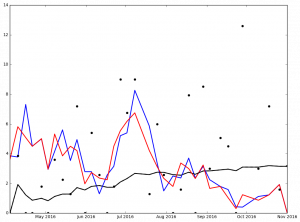
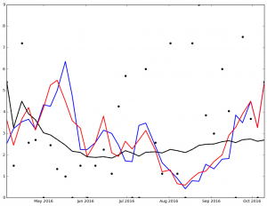
Dr. Drang focused on Jake Arrieta (he is a Chicago guy after all), but I thought it was be interested to look at the Graphs for Arrieta and the top 5 finishers in the NL Cy Young Voting (because Clayton Kershaw was 5th place and I'm a Dodgers guy).

Here is the graph for Jake Arrieata:

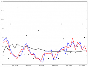
And here are the graphs for the top 5 finishers in Ascending order in the 2016 NL Cy Young voting:

Max Scherzer winner of the 2016 NL Cy Young Award

Jon Lester

Kyle Hendricks

Madison Bumgarner

Clayton Kershaw:

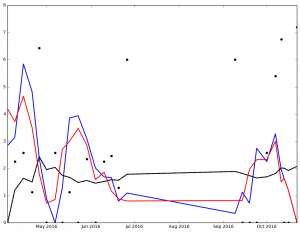
I've not spent much time analyzing the data, but I'm sure that it says something. At the very least, it got me to wonder, 'How many 0 ER games did each pitcher pitch?'

I also noticed that the stats include the playoffs (which I wasn't intending). Another thing to look at later.

Legend:

• Black Dot - ERA on Date of Game
• Black Solid Line - Cumulative ERA
• Blue Solid Line - 3-game trailing average ERA
• Red Solid Line - 4-game trailing average ERA

Full code can be found on my Github Repo

Posted by ryan on Mon 21 November 2016

In Part III I'm reviewing the code to populate a DataFrame with Passer data from the current NFL season.

To start I use the games DataFrame I created in Part II to create 4 new DataFrames:

• reg_season_games - All of the Regular Season Games
• pre_season_games - All of the Pre Season Games
• gameshome - The Home Games
• gamesaway - The Away Games

A cool aspect of the DataFrames is that you can treat them kind of like temporary tables (at least, this is how I'm thinking about them as I am mostly a SQL programmer) and create other temporary tables based on criteria. In the code below I'm taking the nfl_start_date that I defined in Part II as a way to split the data frame into pre / and regular season DataFrame. I then take the regular season DataFrame and split that into home and away DataFrames. I do this so I don't double count the statistics for the passers.

#Start Section 3

reg_season_games = games.loc[games['match_date'] >= nfl_start_date]
pre_season_games = games.loc[games['match_date'] < nfl_start_date]

gameshome = reg_season_games.loc[reg_season_games['ha_ind'] == 'vs']
gamesaway = reg_season_games.loc[reg_season_games['ha_ind'] == '@']

Next, I set up some variables to be used later:

BASE_URL = 'http://www.espn.com/nfl/boxscore/_/gameId/{0}'

#Create the lists to hold the values for the games for the passers
player_pass_name = []
player_pass_catch = []
player_pass_attempt = []
player_pass_yds = []
player_pass_avg = []
player_pass_td = []
player_pass_int = []
player_pass_sacks = []
player_pass_sacks_yds_lost = []
player_pass_rtg = []
player_pass_week_id = []
player_pass_result = []
player_pass_team = []
player_pass_ha_ind = []
player_match_id = []
player_id = [] #declare the player_id as a list so it doesn't get set to a str by the loop below

headers_pass = ['match_id', 'id', 'Name', 'CATCHES','ATTEMPTS', 'YDS', 'AVG', 'TD', 'INT', 'SACKS', 'YRDLSTSACKS', 'RTG']

Now it's time to start populating some of the list variables I created above. I am taking the week_id, result, team_x, and ha_ind columns from the games DataFrame (I'm sure there is a better way to do this, and I will need to revisit it in the future)

player_pass_week_id.append(gamesaway.week_id)
player_pass_result.append(gamesaway.result)
player_pass_team.append(gamesaway.team_x)
player_pass_ha_ind.append(gamesaway.ha_ind)

Now for the looping (everybody's favorite part!). Using BeautifulSoup I get the div of class col column-one gamepackage-away-wrap. Once I have that I get the table rows and then loop through the data in the row to get what I need from the table holding the passer data. Some interesting things happening below:

• The Catches / Attempts and Sacks / Yrds Lost are displayed as a single column each (even though each column holds 2 statistics). In order to fix this I use the index() method and get all of the data to the left of a character (- and / respectively for each column previously mentioned) and append the resulting 2 items per column (so four in total) to 2 different lists (four in total).

The last line of code gets the ESPN player_id, just in case I need/want to use it later.

for index, row in gamesaway.iterrows():
    print(index)
    try:
        request = requests.get(BASE_URL.format(index))
        table_pass = BeautifulSoup(request.text, 'lxml').find_all('div', class_='col column-one gamepackage-away-wrap')

        pass_ = table_pass[0]
        player_pass_all = pass_.find_all('tr')


        for tr in player_pass_all:
            for td in tr.find_all('td', class_='sacks'):
                for t in tr.find_all('td', class_='name'):
                    if t.text != 'TEAM':
                        player_pass_sacks.append(int(td.text[0:td.text.index('-')]))
                        player_pass_sacks_yds_lost.append(int(td.text[td.text.index('-')+1:]))
            for td in tr.find_all('td', class_='c-att'):
                for t in tr.find_all('td', class_='name'):
                    if t.text != 'TEAM':
                        player_pass_catch.append(int(td.text[0:td.text.index('/')]))
                        player_pass_attempt.append(int(td.text[td.text.index('/')+1:]))
            for td in tr.find_all('td', class_='name'):
                for t in tr.find_all('td', class_='name'):
                    for s in t.find_all('span', class_=''):
                        if t.text != 'TEAM':
                            player_pass_name.append(s.text)
            for td in tr.find_all('td', class_='yds'):
                for t in tr.find_all('td', class_='name'):
                    if t.text != 'TEAM':
                        player_pass_yds.append(int(td.text))
            for td in tr.find_all('td', class_='avg'):
                for t in tr.find_all('td', class_='name'):
                    if t.text != 'TEAM':
                        player_pass_avg.append(float(td.text))
            for td in tr.find_all('td', class_='td'):
                for t in tr.find_all('td', class_='name'):
                    if t.text != 'TEAM':
                        player_pass_td.append(int(td.text))
            for td in tr.find_all('td', class_='int'):
                for t in tr.find_all('td', class_='name'):
                    if t.text != 'TEAM':
                        player_pass_int.append(int(td.text))
            for td in tr.find_all('td', class_='rtg'):
                for t in tr.find_all('td', class_='name'):
                    if t.text != 'TEAM':
                        player_pass_rtg.append(float(td.text))
                        player_match_id.append(index)
            #The code below cycles through the passers and gets their ESPN Player ID
            for a in tr.find_all('a', href=True):
                player_id.append(a['href'].replace("http://www.espn.com/nfl/player/_/id/","")[0:a['href'].replace("http://www.espn.com/nfl/player/_/id/","").index('/')])

    except Exception as e:
        pass

With all of the data from above we now populate our DataFrame using specific headers (that's why we set the headers_pass variable above):

player_passer_data = pd.DataFrame(np.column_stack((
player_match_id,
player_id,
player_pass_name,
player_pass_catch,
player_pass_attempt,
player_pass_yds,
player_pass_avg,
player_pass_td,
player_pass_int,
player_pass_sacks,
player_pass_sacks_yds_lost,
player_pass_rtg
)), columns=headers_pass)

An issue that I ran into as I was playing with the generated DataFrame was that even though I had set the numbers generated in the for loop above to be of type int anytime I would do something like a sum() on the DataFrame the numbers would be concatenated as though they were strings (because they were!).

After much Googling I came across a useful answer on StackExchange (where else would I find it, right?)

What it does is to set the data type of the columns from string to int

player_passer_data[['TD', 'CATCHES', 'ATTEMPTS', 'YDS', 'INT', 'SACKS', 'YRDLSTSACKS','AVG','RTG']] = player_passer_data[['TD', 'CATCHES', 'ATTEMPTS', 'YDS', 'INT', 'SACKS', 'YRDLSTSACKS','AVG','RTG']].apply(pd.to_numeric)

OK, so I've got a DataFrame with passer data, I've got a DataFrame with away game data, now I need to join them. As expected, pandas has a way to join DataFrame data ... with the join method obviously!

I create a new DataFrame called game_passer_data which joins player_passer_data with games_away on their common key match_id. I then have to use set_index to make sure that the index stays set to match_id ... If I don't then the index is reset to an auto-incremented integer.

game_passer_data = player_passer_data.join(gamesaway, on='match_id').set_index('match_id')

This is great, but now game_passer_data has all of these extra columns. Below is the result of running game_passer_data.head() from the terminal:

id          Name  CATCHES  ATTEMPTS  YDS  AVG  TD  INT  SACKS

match_id 400874518 2577417 Dak Prescott 22 30 292 9.7 0 0 4 400874674 2577417 Dak Prescott 23 32 245 7.7 2 0 2 400874733 2577417 Dak Prescott 18 27 247 9.1 3 1 2 400874599 2577417 Dak Prescott 21 27 247 9.1 3 0 0 400874599 12482 Mark Sanchez 1 1 8 8.0 0 0 0

           YRDLSTSACKS                        ...

match_id ... 400874518 14 ... 400874674 11 ... 400874733 14 ... 400874599 0 ... 400874599 0 ...

           ha_ind  match_date                  opp result          team_x

match_id 400874518 @ 2016-09-18 washington-redskins W Dallas Cowboys 400874674 @ 2016-10-02 san-francisco-49ers W Dallas Cowboys 400874733 @ 2016-10-16 green-bay-packers W Dallas Cowboys 400874599 @ 2016-11-06 cleveland-browns W Dallas Cowboys 400874599 @ 2016-11-06 cleveland-browns W Dallas Cowboys

          week_id prefix_1             prefix_2               team_y

match_id 400874518 2 wsh washington-redskins Washington Redskins 400874674 4 sf san-francisco-49ers San Francisco 49ers 400874733 6 gb green-bay-packers Green Bay Packers 400874599 9 cle cleveland-browns Cleveland Browns 400874599 9 cle cleveland-browns Cleveland Browns

                                                         url
match_id
400874518  http://www.espn.com/nfl/team/_/name/wsh/washin...
400874674  http://www.espn.com/nfl/team/_/name/sf/san-fra...
400874733  http://www.espn.com/nfl/team/_/name/gb/green-b...
400874599  http://www.espn.com/nfl/team/_/name/cle/clevel...
400874599  http://www.espn.com/nfl/team/_/name/cle/clevel...

That is nice, but not exactly what I want. In order to remove the extra columns I use the drop method which takes 2 arguments:

• what object to drop
• an axis which determine what types of object to drop (0 = rows, 1 = columns):

Below, the object I define is a list of columns (figured that part all out on my own as the documentation didn't explicitly state I could use a list, but I figured, what's the worst that could happen?)

game_passer_data = game_passer_data.drop(['opp', 'prefix_1', 'prefix_2', 'url'], 1)

Which gives me this:

id          Name  CATCHES  ATTEMPTS  YDS  AVG  TD  INT  SACKS

match_id 400874518 2577417 Dak Prescott 22 30 292 9.7 0 0 4 400874674 2577417 Dak Prescott 23 32 245 7.7 2 0 2 400874733 2577417 Dak Prescott 18 27 247 9.1 3 1 2 400874599 2577417 Dak Prescott 21 27 247 9.1 3 0 0 400874599 12482 Mark Sanchez 1 1 8 8.0 0 0 0

           YRDLSTSACKS    RTG ha_ind  match_date result          team_x

match_id 400874518 14 103.8 @ 2016-09-18 W Dallas Cowboys 400874674 11 114.7 @ 2016-10-02 W Dallas Cowboys 400874733 14 117.4 @ 2016-10-16 W Dallas Cowboys 400874599 0 141.8 @ 2016-11-06 W Dallas Cowboys 400874599 0 100.0 @ 2016-11-06 W Dallas Cowboys

          week_id               team_y
match_id
400874518       2  Washington Redskins
400874674       4  San Francisco 49ers
400874733       6    Green Bay Packers
400874599       9     Cleveland Browns
400874599       9     Cleveland Browns

I finally have a DataFrame with the data I care about, BUT all of the column names are wonky!

This is easy enough to fix (and should have probably been fixed earlier with some of the objects I created only containing the necessary columns, but I can fix that later). By simply renaming the columns as below:

game_passer_data.columns = ['id', 'Name', 'Catches', 'Attempts', 'YDS', 'Avg', 'TD', 'INT', 'Sacks', 'Yards_Lost_Sacks', 'Rating', 'HA_Ind', 'game_date', 'Result', 'Team', 'Week', 'Opponent']

I now get the data I want, with column names to match!

id          Name  Catches  Attempts  YDS  Avg  TD  INT  Sacks

match_id 400874518 2577417 Dak Prescott 22 30 292 9.7 0 0 4 400874674 2577417 Dak Prescott 23 32 245 7.7 2 0 2 400874733 2577417 Dak Prescott 18 27 247 9.1 3 1 2 400874599 2577417 Dak Prescott 21 27 247 9.1 3 0 0 400874599 12482 Mark Sanchez 1 1 8 8.0 0 0 0

           Yards_Lost_Sacks  Rating HA_Ind   game_date Result            Team

match_id 400874518 14 103.8 @ 2016-09-18 W Dallas Cowboys 400874674 11 114.7 @ 2016-10-02 W Dallas Cowboys 400874733 14 117.4 @ 2016-10-16 W Dallas Cowboys 400874599 0 141.8 @ 2016-11-06 W Dallas Cowboys 400874599 0 100.0 @ 2016-11-06 W Dallas Cowboys

          Week             Opponent
match_id
400874518    2  Washington Redskins
400874674    4  San Francisco 49ers
400874733    6    Green Bay Packers
400874599    9     Cleveland Browns
400874599    9     Cleveland Browns

I've posted the code for all three parts to my GitHub Repo.

Work that I still need to do:

1. Add code to get the home game data
2. Add code to get data for the other position players
3. Add code to get data for the defense

When I started this project on Wednesday I had only a bit of exposure to very basic aspects of Python and my background as a developer. I'm still a long way from considering myself proficient in Python but I know more now that I did 3 days ago and for that I'm pretty excited! It's also given my an ~~excuse~~ reason to write some stuff which is a nice side effect.

Posted by ryan on Sat 19 November 2016

On a previous post I went through my new found love of Fantasy Football and the rationale behind the 'why' of this particular project. This included getting the team names and their URLs from the ESPN website.

As before, let's set up some basic infrastructure to be used later:

from time import strptime

year = 2016 # allows us to change the year that we are interested in.
nfl_start_date = date(2016, 9, 8)
BASE_URL = 'http://espn.go.com/nfl/team/schedule/_/name/{0}/year/{1}/{2}' #URL that we'll use to cycle through to get the gameid's (called match_id)

match_id = []
week_id = []
week_date = []
match_result = []
ha_ind = []
team_list = []

Next, we iterate through the teams dictionary that I created yesterday:

for index, row in teams.iterrows():
    _team, url = row['team'], row['url']
    r=requests.get(BASE_URL.format(row['prefix_1'], year, row['prefix_2']))
    table = BeautifulSoup(r.text, 'lxml').table
    for row in table.find_all('tr')[2:]: # Remove header
        columns = row.find_all('td')
        try:
            for result in columns[3].find('li'):
                match_result.append(result.text)
                week_id.append(columns[0].text) #get the week_id for the games dictionary so I know what week everything happened
                _date = date(
                    year,
                    int(strptime(columns[1].text.split(' ')[1], '%b').tm_mon),
                    int(columns[1].text.split(' ')[2])
                )
                week_date.append(_date)
                team_list.append(_team)
                for ha in columns[2].find_all('li', class_="game-status"):
                    ha_ind.append(ha.text)
            for link in columns[3].find_all('a'): # I realized here that I didn't need to do the fancy thing from the site I was mimicking http://danielfrg.com/blog/2013/04/01/nba-scraping-data/
                match_id.append(link.get('href')[-9:])

        except Exception as e:
            pass

Again, we set up some variables to be used in the for loop. But I want to really talk about the try portion of my code and the part where the week_date is being calculated.

Although I've been developing and managing developers for a while, I've not had the need to use a construct like try. (I know, right, weird!)

The basic premise of the try is that it will execute some code and if it succeeds that code will be executed. If not, it will go to the exception portion. For Python (and maybe other languages, I'm not sure) the exception MUST have something in it. In this case, I use Python's pass function, which basically says, 'hey, just forget about doing anything'. I'm not raising any errors here because I don't care if the result is 'bad' I just want to ignore it because there isn't any data I can use.

The other interesting (or gigantic pain in the a\$\$) thing is that the way ESPN displays dates on the schedule page is as Day of Week, Month Day, i.e. Sun Sep 11. There is no year. I think this is because for the most part the regular season for an NFL is always in the same calendar year. However, this year the last game of the season, in week 17, is in January. Since I'm only getting games that have been played, I'm safe for a couple more weeks, but this will need to be addressed, otherwise the date of the last games of the 2016 season will show as January 2016, instead of January 2017.

Anyway, I digress. In order to change the displayed date to a date I can actually use is I had to get the necessary function. In order to get that I had to add the following line to my code from yesterday

from time import strptime

This allows me to make some changes to the date (see where _date is being calculated in for result in columns[3].find('li'): portion of the try:.

One of the things that confused the heck out of me initially was the way the date is being stored in the list week_date. It is in the form datetime.date(2016, 9, 1), but I was expecting it to be stored as 2016-09-01. I did a couple of things to try and fix this, especially because once the list was added to the gamesdic dictionary and then used in the games DataFrame the week_date was then stored as 1472688000000 which is the milliseconds since Jan 1, 1970 to the date of the game, but it took an embarising amount of Googling to ~~realize~~ discover this.

With this new discovery, I forged on. The last two things that I needed to do was to create a dictionary to hold my data with all of my columns:

gamesdic = {'match_id': match_id, 'week_id': week_id, 'result': match_result, 'ha_ind': ha_ind, 'team': team_list, 'match_date': week_date}

With dictionary in hand I was able to create a DataFrame:

games = pd.DataFrame(gamesdic).set_index('match_id')

The line above is frighteningly simple. It's basically saying, hey, take all of the data from the gamesdic dictionary and make the match_id the index.

To get the first part, see my post Web Scrapping - Passer Data (Part I).

Posted by ryan on Fri 18 November 2016

For the first time in many years I've joined a Fantasy Football league with some of my family. One of the reasons I have not engaged in the Fantasy football is that, frankly, I'm not very good. In fact, I'm pretty bad. I have a passing interest in Football, but my interests lie more with Baseball than football (especially in light of the NFLs policy on punishing players for some infractions of league rules, but not punishing them for infractions of societal norms (see Tom Brady and Ray Lewis respectively).

That being said, I am in a Fantasy Football league this year, and as of this writing am a respectable 5-5 and only 2 games back from making the playoffs with 3 games left.

This means that what I started on yesterday I really should have started on much sooner, but I didn't.

I had been counting on ESPN's 'projected points' to help guide me to victory ... it's working about as well as flipping a coin (see my record above).

I had a couple of days off from work this week and some time to tinker with Python, so I thought, what the hell, let's see what I can do.

Just to see what other people had done I did a quick Google Search and found someone that had done what I was trying to do with data from the NBA in 2013.

Using their post as a model I set to work.

The basic strategy I am mimicking is to:

• Get the Teams and put them into a dictionary
• Get the 'matches' and put them into a dictionary
• Get the player stats and put them into a dictionary for later analysis

I start of importing some standard libraries pandas, requests, and BeautifulSoup (the other libraries are for later).

import pandas as pd
import requests
from bs4 import BeautifulSoup
import csv
import numpy as np
from datetime import datetime, date

Next, I need to set up some variables. BeautifulSoup is a Python library for pulling data out of HTML and XML files.. It's pretty sweet. The code below is declaring a URL to scrape and then users the requests library to get the actual HTML of the page and put it into a variable called r.

url = 'http://espn.go.com/nfl/teams'
r = requests.get(url)

r has a method called text which I'll use with BeautifulSoup to create the soup. The 'lxml' declares the parser type to be used. The default is lxml and when I left it off I was presented with a warning, so I decided to explicitly state which parser I was going to be using to avoid the warning.

soup = BeautifulSoup(r.text, 'lxml')

Next I use the find_all function from BeautifulSoup. The cool thing about find_all is that you can either pass just a tag element, i.e. li or p, but you can add an additional class_ argument (notice the underscore at the end ... I missed it more than once and got an error because class is a keyword used by Python). Below I'm getting all of the `ul' elements of the class type 'medium-logos'.

tables = soup.find_all('ul', class_='medium-logos')

Now I set up some list variables to hold the items I'll need for later use to create my dictionary

teams = []
prefix_1 = []
prefix_2 = []
teams_urls = []

Now, we do some actual programming:

Using a nested for loop to find all of the li elements in the variable called lis which is based on the variable tables (recall this is all of the HTML from the page I scrapped that has only the tags that match <ul class='medium-logos></ul> and all of the content between them).

The nested for loop creates 2 new variables which are used to populate the 4 lists from above. The creating of the info variable gets the a tag from the li tags. The url variable takes the href tag from the info variable. In order to add an item to a list (remember, all of the lists above are empty at this point) we have to invoke the method append on each of the lists with the data that we care about (as we look through).

The function split can be used on a string (which url is). It allows you to take a string apart based on a passed through value and convert the output into a list. This is super useful with URLs since there are many cases where we're trying to get to the path. Using split('/') allows the URL to be broken into it's constituent parts. The negative indexes used allows you to go from right to left instead of left to right.

To really break this down a bit, if we looked at just one of the URLs we'd get this:

http://www.espn.com/nfl/team/_/name/ten/tennessee-titans

The split('/') command will turn the URL into this:

['http:', '', 'www.espn.com', 'nfl', 'team', '_', 'name', 'ten', 'tennessee-titans']

Using the negative index allows us to get the right most 2 values that we need.

for table in tables:
    lis = table.find_all('li')
    for li in lis:
        info = li.h5.a
        teams.append(info.text)
        url = info['href']
        teams_urls.append(url)
        prefix_1.append(url.split('/')[-2])
        prefix_2.append(url.split('/')[-1])

Now we put it all together into a dictionary

dic = {'url': teams_urls, 'prefix_2': prefix_2, 'prefix_1': prefix_1, 'team': teams}
teams = pd.DataFrame(dic)

This is the end of part 1. Parts 2 and 3 will be coming later this week.

I've also posted all of the code to my GitHub Repo.

Posted by ryan on Fri 18 November 2016

Nothing can ever really be considered done when you're talking about programming, right?

I decided to try and add images to the python script I wrote last week and was able to do it, with not too much hassel.

The first thing I decided to do was to update the code on pythonista on my iPad Pro and verify that it would run.

It took some doing (mostly because I forgot that the attributes in an img tag included what I needed ... initially I was trying to programmatically get the name of the person from the image file itelf using regular expressions ... it didn't work out well).

Once that was done I branched the master on GitHub into a development branch and copied the changes there. Once that was done I performed a pull request on the macOS GitHub Desktop Application.

Finally, I used the macOS GitHub app to merge my pull request from development into master and now have the changes.

The updated script will now also get the image data to display into the multi markdown table:

| Name | Title | Image |
| --- | --- | --- |
|Mike Cheley|CEO/Creative Director|![alt text](https://www.graphtek.com/user_images/Team/Mike_Cheley.png "Mike Cheley")|
|Ozzy|Official Greeter|![alt text](https://www.graphtek.com/user_images/Team/Ozzy.png "Ozzy")|
|Jay Sant|Vice President|![alt text](https://www.graphtek.com/user_images/Team/Jay_Sant.png "Jay Sant")|
|Shawn Isaac|Vice President|![alt text](https://www.graphtek.com/user_images/Team/Shawn_Isaac.png "Shawn Isaac")|
|Jason Gurzi|SEM Specialist|![alt text](https://www.graphtek.com/user_images/Team/Jason_Gurzi.png "Jason Gurzi")|
|Yvonne Valles|Director of First Impressions|![alt text](https://www.graphtek.com/user_images/Team/Yvonne_Valles.png "Yvonne Valles")|
|Ed Lowell|Senior Designer|![alt text](https://www.graphtek.com/user_images/Team/Ed_Lowell.png "Ed Lowell")|
|Paul Hasas|User Interface Designer|![alt text](https://www.graphtek.com/user_images/Team/Paul_Hasas.png "Paul Hasas")|
|Alan Schmidt|Senior Web Developer|![alt text](https://www.graphtek.com/user_images/Team/Alan_Schmidt.png "Alan Schmidt")|

Which gets displayed as this:

Name Title Image

Mike Cheley CEO/Creative Director Ozzy Official Greeter Jay Sant Vice President Shawn Isaac Vice President Jason Gurzi SEM Specialist Yvonne Valles Director of First Impressions Ed Lowell Senior Designer Paul Hasas User Interface Designer Alan Schmidt Senior Web Developer

Posted by ryan on Sat 22 October 2016